Integrating Monte Carlo Tree Search and Neural Networks

Tue Jul 03 2018

Series: Monte Carlo Tree Search

My last post covered Monte Carlo Tree Search in its “vanilla” form. It’s a fantastic algorithm for tackling games with high branching factors - but there is a slight problem. Vanilla MCTS follows a “light rollout” policy - once MCTS encounters a game state that it’s never seen, it explores at random. This means we may under-explore important lines of play. We try to solve for this by simulating lots of times, but this solution isn’t perfect; in games with a large number of game states, we’re certain to needlessly explore obviously wrong choices (and probably miss a lot of great ones).

Humans deal with this through intuition. A human who’s played a lot of chess will look at a chess position and see a couple moves that are obviously interesting, and there’s a lot of moves they wouldn’t consider because they’re obviously not worth thinking about. This post aims to show how we “humanize” our MCTS; we’ll show how we can improve our performance immensely by arming our tree search with a neural network for guidance, and how we can use our tree search to train that neural network along the way.

Preface

The majority of the methods described in this article were taken from the AlphaGo Zero paper ”Mastering the Game of Go without Human Knowledge”. There are many plausible modifications that could be made to these methods that could still result in the successful integration neural nets and MCTS.

This article is focused on covering how to combine MCTS and neural nets, rather than what they are. It’s recommended that readers have read my previous post on vanilla Monte Carlo Tree Search and that they have a functional knowledge of neural nets before tackling the concepts in this post. If you need a quick primer on neural nets, check out this post. Now let’s get into it!

The Neural Net

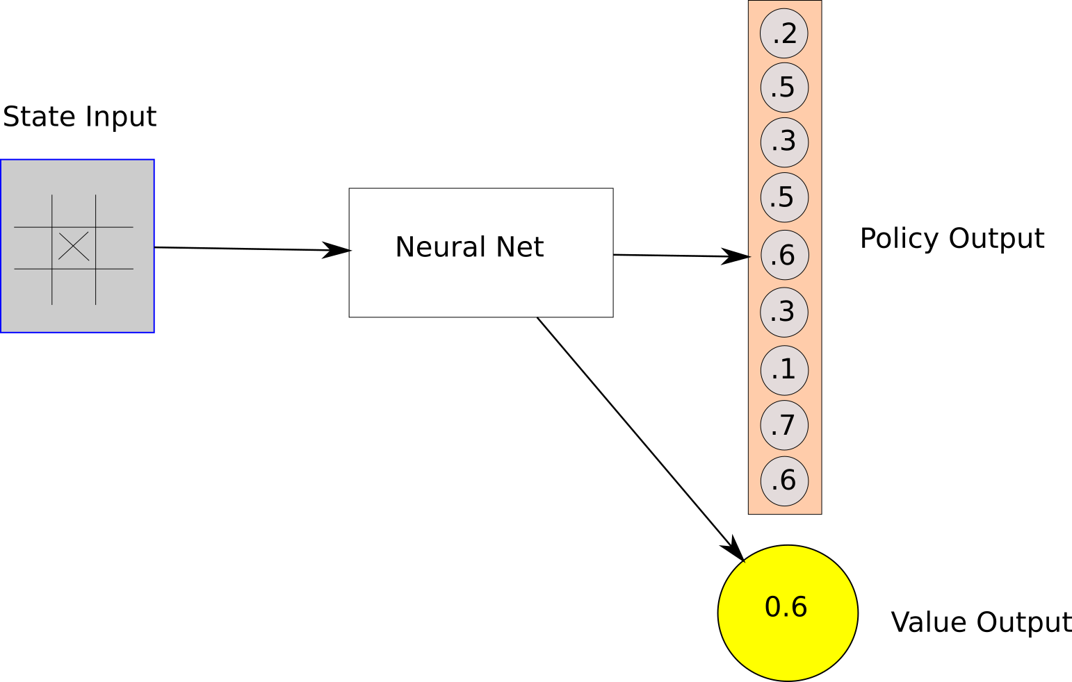
The neural net in our discussion has two outputs - a policy output and a value output. This means that for any game state or board position, the neural net will output a policy vector and a value. The policy vector will be a list of numbers, each number giving the logit probability of choosing a particular action. The value is a real number between -1 and 1 which represents the likelihood that the agent will win from that state. (1 is a win, -1 is a loss and 0 is a draw.) We should note that it is possible to integrate MCTS with neural nets that have different architectures. It’s possible use a neural net that just has a policy output, or two different neural nets for policy and value (this was the original AlphaGo design!)

Using a Neural Net to Guide MCTS

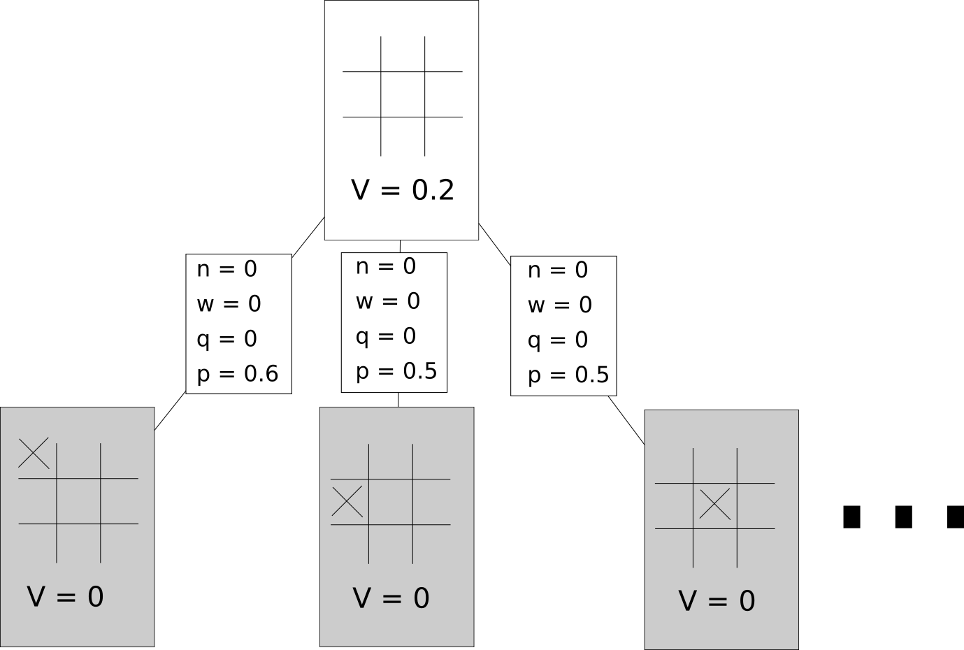
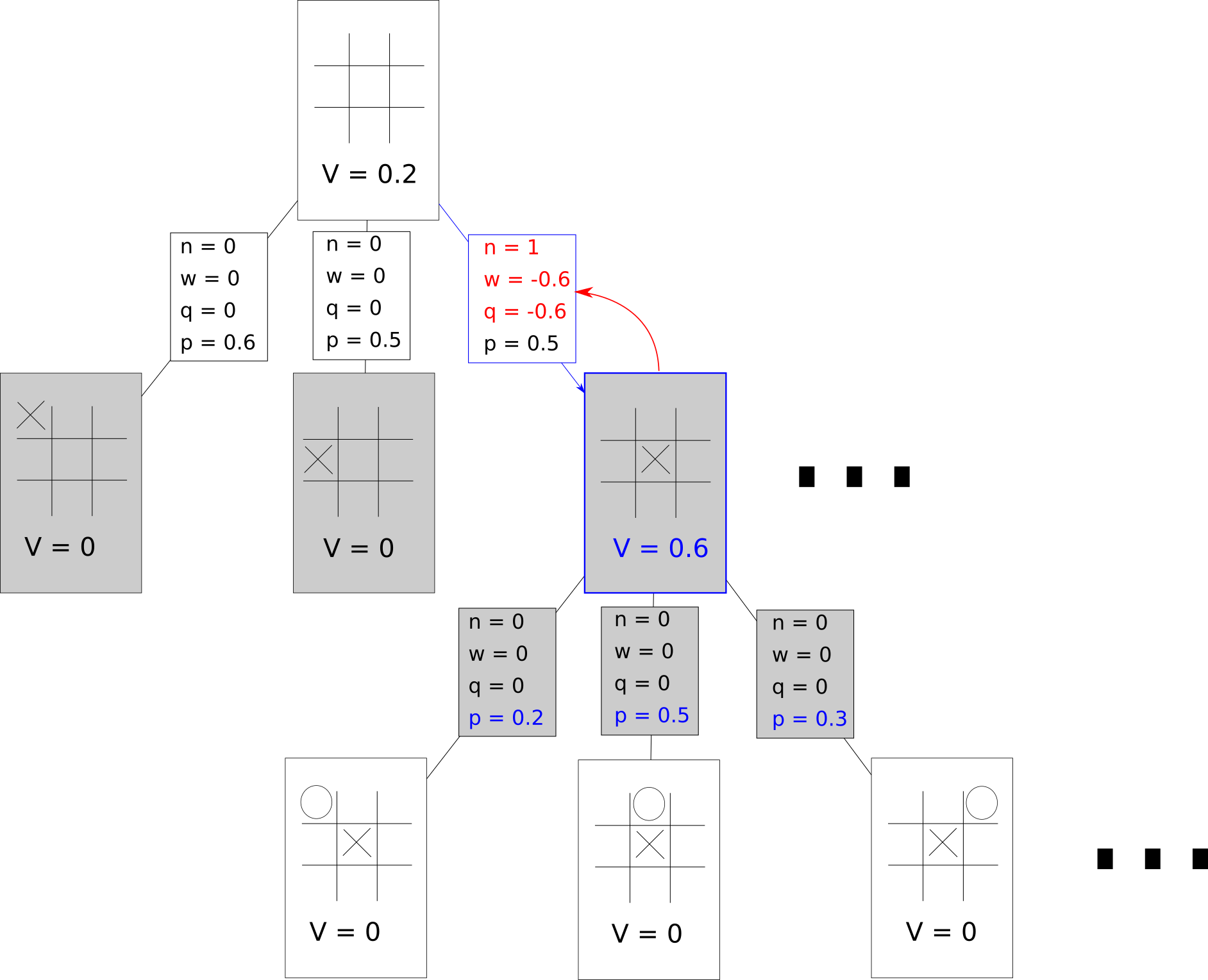
Let’s revisit HAL, our AI agent that’s using Monte Carlo Tree Search With “vanilla” monte-carlo tree search, the nodes keep track of the visit count and the win count. In this version, it’s easier to think of the edges doing most of the tracking. Instead of a visit count and win count, they will track the visit count $n$ , a prior probability $p$ , an intermediary value $w$ , and an action-value $q$ . The nodes do store a “state value”. A graphical representation of this might look like this hypothetical game tree early on in the tree search:

Some Terminology

We’ll represent the visit count of a given game state $s$ and an associated action $a$ as $N(s, a)$ The prior probability of a taking an action from a game state will be represented as $P(s, a)$ . For any state, the prior probabilities for all actions are given by our neural network. The action-value of a given action will be represents as $Q(s, a)$ . This represents the value of taking that action, and it’s reasonable to think of this as analogous to the win-count / visit-count metric in regular MCTS. How this is calculated will be covered later in the article. In this discussion, we’ll stick to using tic-tac-toe as our example game environment for simplicity, but this algorithm is of course intended to be used on far more complex game environments.

Selection Phase

In the selection phase, we face the same dilemma as in the regular Monte-Carlo Tree Search - we want to make sure we explore deeply into nodes that are promising, but we also want to make sure we’re exploring nodes that haven’t been explored very much. How do we choose which action to think about taking? Recall that in the vanilla MCTS algorithm we showed how this could be accomplished with the UCB1 formula. That formula doesn’t quite work if we want to account for the recommendations of our neural net, though. Instead, we can select the action that maximizes the following equation:

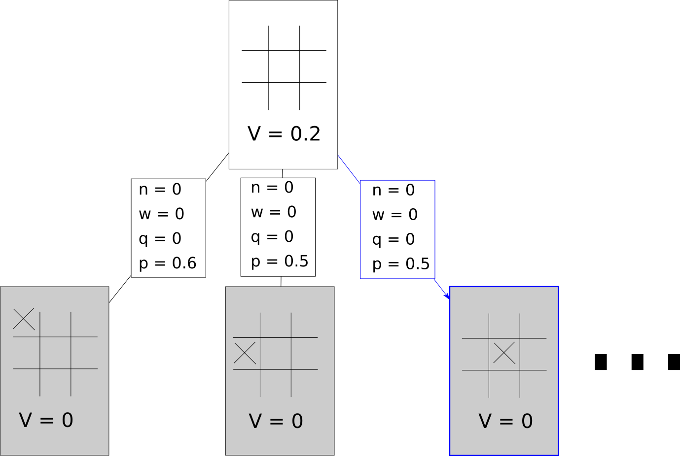
Q(s, a) + c_{puct}P(s, a)\frac{\sqrt{\sum_b N(s, b)}}{1 + N(s, a)}

This formula is actually very similar to UCB1. $c$ is still an exploration parameter - the higher this is set, the more we prefer exploring new knowledge to exploiting current knowledge. We also have the option of adding Dirichlet noise to our priors. This allows for some level of randomness in the selection process, but very strong priors will still overrule that randomness. This was applied only in the root node in AlphaGo. We’ll assume that based on the above equation with some added Dirichlet noise, we choose the following node.

Expansion/Evaluation Phase

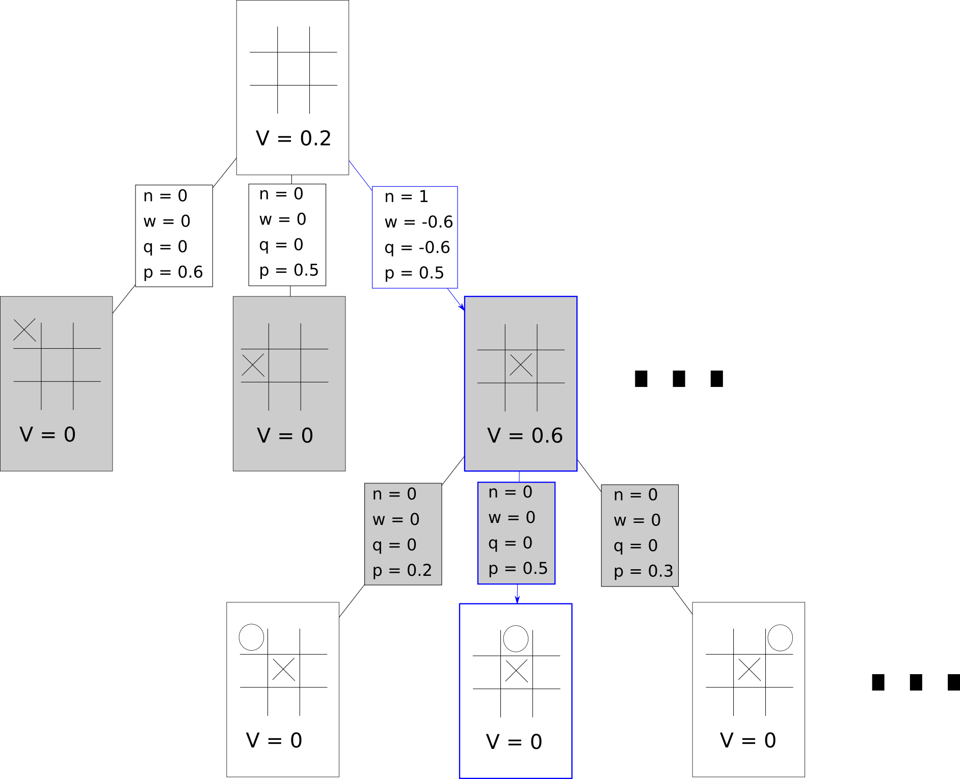
The node that we chose is a leaf node. Leaf nodes have zero-values and no edges.When a leaf node is encountered, we evaluate the state using a neural network and get a vector of action-probabilities $p\_a$ and a value $v$ .

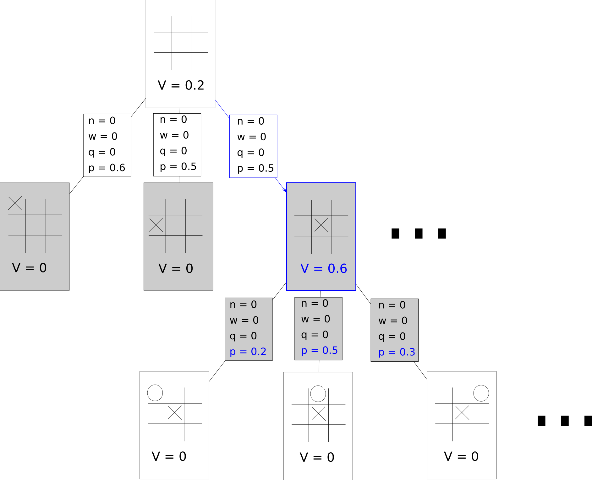
In this hypothetical scenario, our neural net has predicted a state value of 0.6. It’s also given us a list of nine logit probabilities for our possible nine actions. These numbers give us the prior probabilities of our edges.

Note: Our neural net will always output a vector of nine numbers, corresponding to nine boxes where we might play in tic-tac-toe. In some states, not all of these actions are valid - for example, we can’t play in the center square if our opponent has already played in the center square. Making sure we only choose from valid actions is a job for the MCTS algorithm implementation.

After this evaluation, the game tree looks like this:

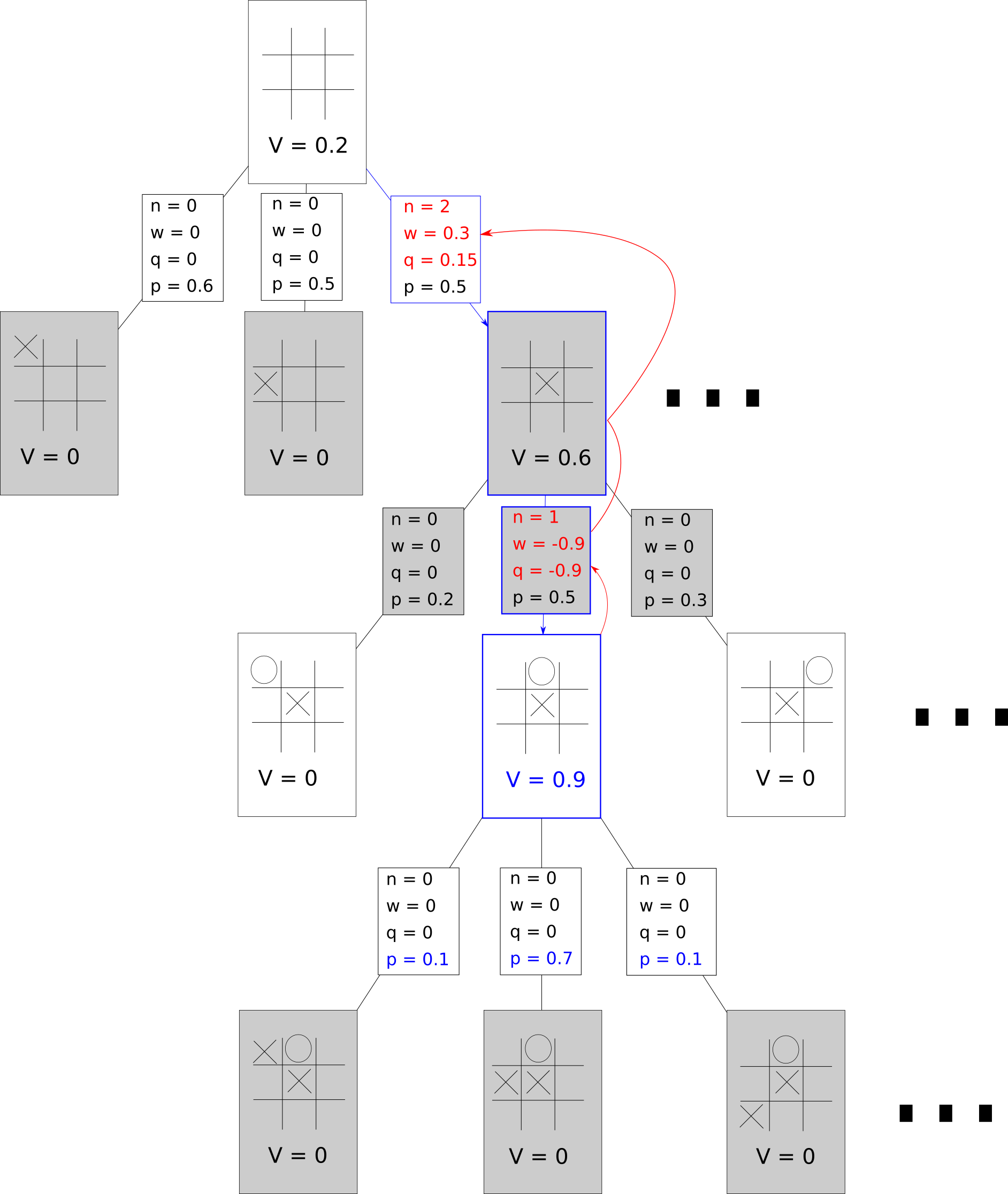
Update

For every edge $e_t$ that was traversed up until the recently expanded leaf node, three updates are performed.

1. The visit count is incremented.

2. If the player that owns $e_t$ is the same player that owns the leaf node, then we add $v$ to $w \!$ . Otherwise, we subtract $v$ from $w \!$ .

3. We update the action-value q to w/n.

Repeat!

This is done over and over again until our computation time has run out. Just for the sake of example, we’ll quickly go through what one more update might look like. Note that the nodes selected do not necessarily reflect what the PUCT algorithm would actually select.

Select with PUCT Until a Leaf Node

Expand and Evaluate the Leaf Node

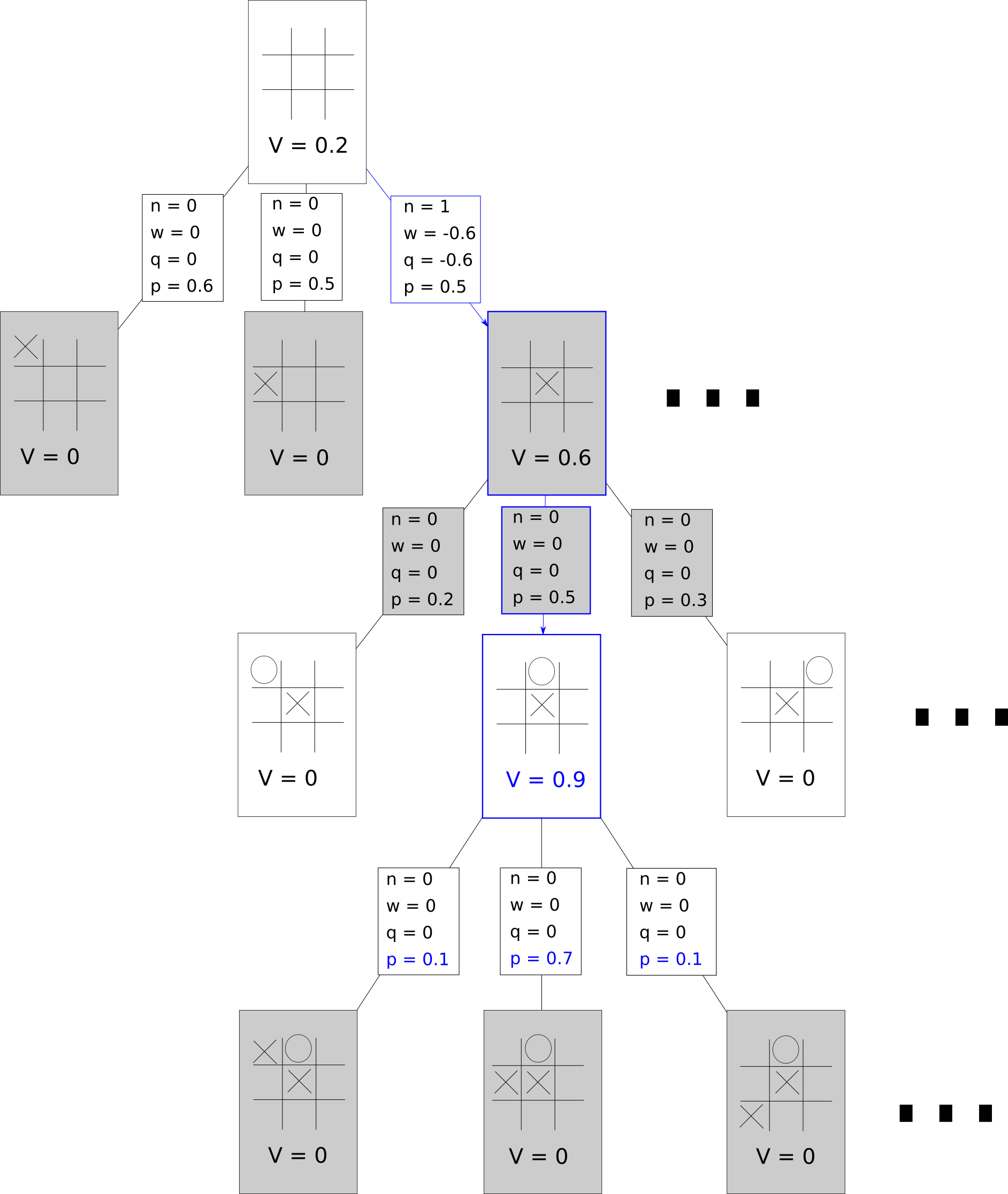
Update All Traversed Edges according to the value of the leaf node.

Choosing an Action

After the steps above have been repeated many times, we’ll have a pretty big game tree. All we need to do now is choose which move we actually want to play! We generate a list of probabilities of choosing a given action according to this formula.

\pi_t = N(s, a)^{1/t}/\sum_b N(s, b)^{1/t}

The temperature parameter $t$ describes how much you want to value the visit count of a given edge. The closer to zero this is set, the more chance there is of choosing greedily with respect to visit count, where a temperature parameter of one will more readily choose less-explored actions.

Using MCTS Results as Training Data

We’ve covered how we can use a neural net in conjunction with MCTS, but how do we make sure the neural net keeps improving with constant play?

After playing an entire game against itself using MCTS, we generate some datapoints.

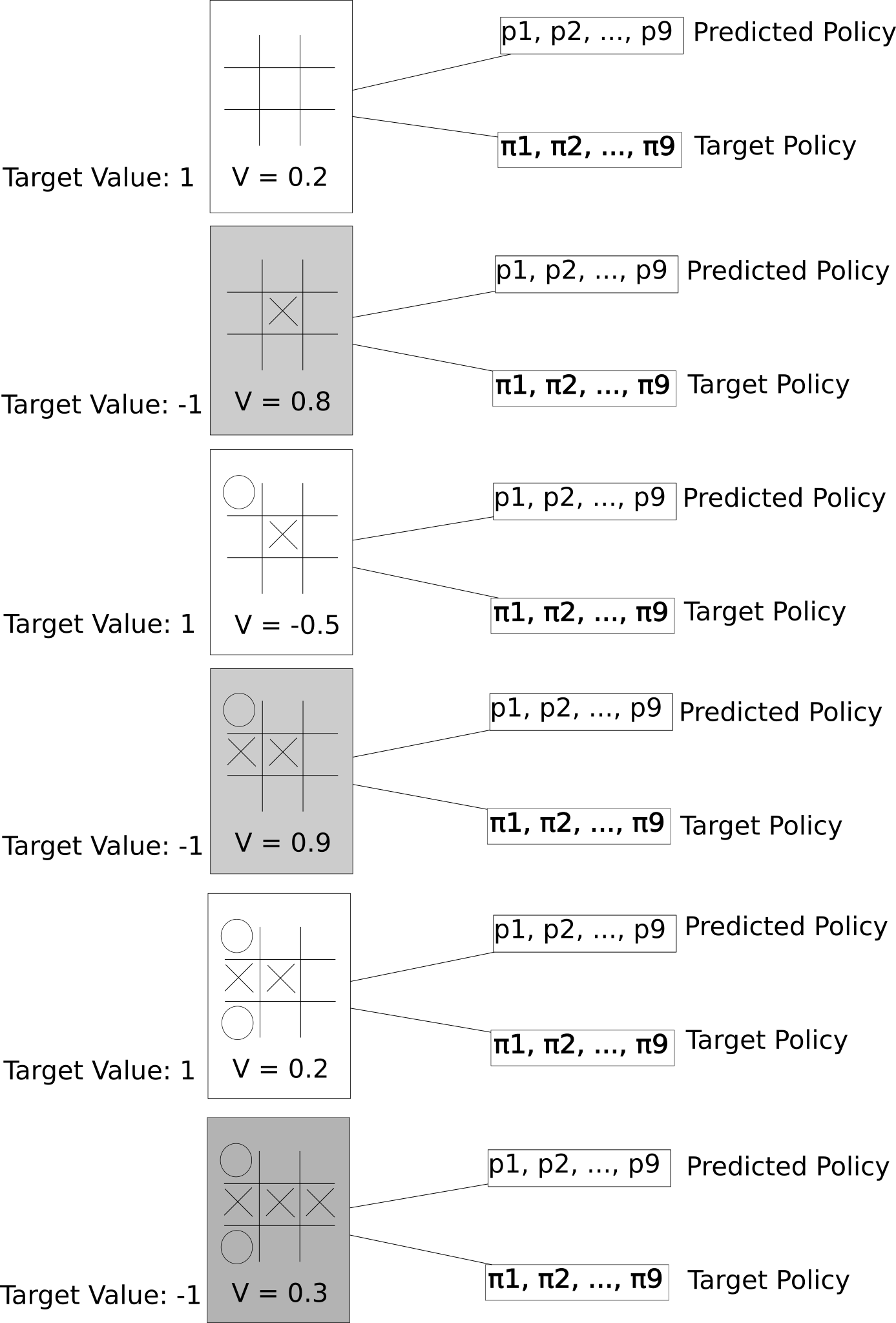
Each move we’ve played has an input state, a target value (depending on who won), a predicted value, a predicted policy (the prior probabilities of each edge), and a target policy (the search probabilities of each edge). This is all we need to train our neural net.

Important Note

We shouldn’t be constantly training the neural network that’s guiding our MCTS and generating our data. Instead, we have two neural networks - our data generation network and our training network. The data generation network is what we actually use in our MCTS simulations. This network generates new data for the training network to learn from. After a set number of training steps (1000 for AlphaGo Zero), an MCTS using our training network is pitted against one with our data generation network in a tournament. If the data generation network loses, it gets replaced by our training network.